A Loading Expression Data in R
A.1 Exploring the Available Project Data
Whether you’ve found a dataset through the SRA or GEO, we want to get the data into R to start working with it. For now, we will only download the count data which is most likely stored in a TXT or XLS(X) file format:
Data formats:
-
TXT: simple text file containing a minimum of two columns (either tab or comma separated containing i.e. gene / transcript identifier and one of the above mentioned data types).
- However it can also contain up to 10 data columns either including more information regarding the gene/ transcript (i.e. gene ID, name, symbol, chromosome, start/ stop position, length, etc.) or more numerical columns (i.e. raw read count, normalized readcount, FPKM, etc.).
- XLS(X): Microsoft Excel file containing the same data columns as mentioned in the TXT files.
Data types:
- Read Count (required; simple raw count of mapped reads to a certain gene or transcript).
- FPKM (Fragments Per Kilobase Million, F for Fragment, paired-end sequencing),
- RPKM (Reads Per Kilobase Million, R for Read, single-end sequencing),
- TPM (Transcripts Per Kilobase Million, T for Transcript, technique independent),
Layouts
- Either one or more files per sample with one of the above data types or
- One file containing the data types for all samples (with the samples as data columns in the file)
Please watch the video and read the page found at the RNA-Seq blog regarding the meaning and calculation of the above mentioned expression data formats or a more technical document found at The farrago blog page.
On GEO you can see what data might be availalbe in the Supplementary column, as shown below:

Figure A.1: Finding an experiment on GEO with a TXT file as supplementary data
This overview on GEO contains many links which are not direct links to the items for that dataset, but can be used as filter for browsing the results. If you want to actually download the data, click on the GSE identifier (first column) which brings you to an overview for this experiment containing a lot of information about the experiment (subject, research institute, publication, design, etc.) and links to each individual sample (GSM identifier). Following the link to a sample shows information on how this sample was retrieved with often many (lab) protocols used. Sometimes there is a segment regarding “Data Processing” that refers to techniques and software used for the full analysis and might contain something like:
… Differential expression testing between sample groups was performed in Rstudio (v. 1.0.36) using DESeq2 (v.1.14.1) …
Back on the experiment overview page you’ll see a (variable) number of links to data files belonging to this experiment, see \(\ref{fig:GEO_Data-download}\). For now we are only interested in the count-data which is stored in the TXT-file (see the column File type/resource) called GSE97406_RAW.tar. This file contains all the data that we need, even though it is only 220Kb in size where the experiment started with about 5Gb of read-data for a small bacteria:
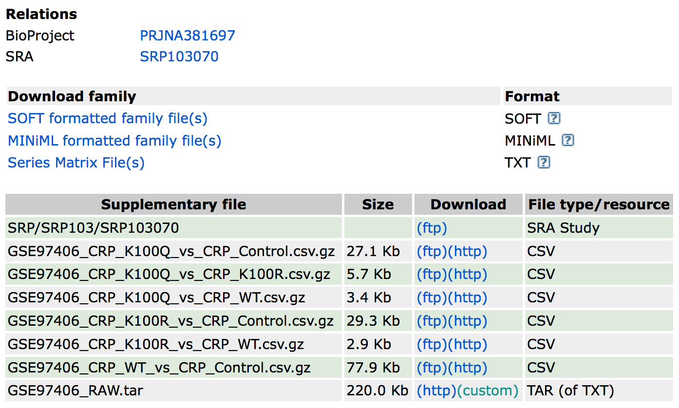
Figure A.2: Finding the supplementary data in a GEO record
As a bioinformatician we love to compress all the files so for this particular example, we download the tar-archive file, extract it to find a folder with another archive file for each sample. After extracting these files we end up with 12 TXT-files with just two columns; a gene identifier and a raw count value (~4500 rows of data per sample):
| Gene ID | Count Value |
|---|---|
| aaaD | 0 |
| aaaE | 0 |
| aaeR | 50 |
| aaeX | 0 |
| aas | 118 |
| abgB | 21 |
| abgR | 56 |
| abgT | 0 |
| abrB | 11 |
| accA | 453 |
| accB | 2492 |
| accC | 1197 |
Other experiments combine their samples in a single file where each column represents a sample. If you do get an experiment with one file per sample, we can programmatically (yes, even in R) load this data in batch.
A.2 Batch Loading Expression Data
This code example shows how to batch-load multiple files containing expression (count) data for a single sample. The data for this example can be found on GEO with ID GSE109798. Downloading the data for this experiment from GEO gives us a single .tar file called GSE109798_RAW.tar. Extracting this archive file nets us a folder with the following files:
file.names <- list.files('./data/GSE109798_RAW/')| Files |
|---|
| GSM2970149_4T1E274.isoforms.results.txt |
| GSM2970150_4T1E266.isoforms.results.txt |
| GSM2970151_4T1E247D.isoforms.results.txt |
| GSM2970152_4T1P2247A.isoforms.results.txt |
| GSM2970153_4T1P2247G.isoforms.results.txt |
| GSM2970154_4T1P2247F.isoforms.results.txt |
| GSM2970155_HCC1806E224B.isoforms.results.txt |
| GSM2970156_HCC1806E224A.isoforms.results.txt |
| GSM2970157_HCC1806E224C.isoforms.results.txt |
| GSM2970158_HCC1806P2232A.isoforms.results.txt |
| GSM2970159_HCC1806P2232B.isoforms.results.txt |
| GSM2970160_HCC1806P2230.isoforms.results.txt |
A.2.1 Decompressing
The file extension of all these files is .txt.gz which means that all files are compressed using gzip and need to be unpacked before they can be loaded. The easiest method is using the system gunzip command on all files which can be done from within R by applying the gunzip command using the system function on each file.
## Change directory to where the files are stored
setwd('./data/GSE109798_RAW/')
sapply(file.names, FUN = function(file.name) {
  system(paste("gunzip", file.name))
  })
Now we can update the file.names variable since each file name has changed.
file.names <- list.files('./data/GSE109798_RAW/')A.2.2 Determining Data Format
Next, we can inspect what the contents are of these files, assuming that they all have the same layout/ column names etc. to decide what we need to use for our analysis.
## Call the system 'head' tool to 'peek' inside the file
system(paste0("head ", "./data/GSE109798_RAW/", file.names[1]))| transcript_id | gene_id | length | effective_length | expected_count | TPM | FPKM | IsoPct |
|---|---|---|---|---|---|---|---|
| uc007aet.1 | 1 | 3608 | 3608.00 | 1.82 | 0.44 | 0.24 | 100.00 |
| uc007aeu.1 | 1 | 3634 | 3634.00 | 0.00 | 0.00 | 0.00 | 0.00 |
| uc011whv.1 | 10 | 26 | 26.00 | 0.00 | 0.00 | 0.00 | 0.00 |
| uc007amd.1 | 100 | 1823 | 1823.00 | 0.00 | 0.00 | 0.00 | 0.00 |
| uc007ame.1 | 100 | 4355 | 4355.00 | 1.32 | 0.26 | 0.15 | 100.00 |
| uc007dac.1 | 1000 | 1403 | 1403.00 | 2.00 | 1.25 | 0.70 | 100.00 |
| uc008ajp.1 | 10000 | 1078 | 1078.00 | 0.00 | 0.00 | 0.00 | 0.00 |
| uc012ajs.1 | 10000 | 1753 | 1753.00 | 0.00 | 0.00 | 0.00 | 0.00 |
| uc008ajq.1 | 10001 | 2046 | 2046.00 | 0.00 | 0.00 | 0.00 | 0.00 |
These files contain (much) more then just a count value for each gene as we can see columns such as (transcript) length, TPM, FPKM, etc. Also, the count-column is called expected_count which raises a few questions as well.
The expected count value is usable as it contains more
information - compared to the raw count - then we actually require. The
expected part results from multimapped reads where a
single read mapped to multiple positions in the genome. As each
transcript originates only from one location, this multimapped read is
usually discarded. With the expected count though, instead of
discarding the read completely it is estimated where it
originates from and this is added as a fraction to the count
value. So the value of 1.32 that we see on line 5 in the
example above means an true count of 1 (uniquely mapped
read) and the .32 (the estimated part) results from an
algorithm and can mean multiple things.
As mentioned before, we require integer count data for use with
packages such as DESeq2 and edgeR and there
are two methods to convert the expected count to raw count data: +
round the value to the nearest integer (widely accepted method
and is well within the expected sampling variation), or + discard the
fraction part by using for example the floor()
function.
A.2.3 Loading Data
From all these columns we want to keep the transcript_id and expected_count columns and ignore the rest (we might be interested in this data later on though). As we need to lead each file separately we can define a function that reads in the data, keeping the columns of interest and returning a dataframe with this data. Note that the first line of each file is used as a header, but check before setting the header argument to TRUE, sometimes the expression data starts at line 1. The file name is then also used to name the column in the dataframe so that we know which column is which sample. This is done by splitting the file name (using strsplit) using the dot (‘.’) keeping the first part (i.e. ‘GSM2970156_HCC1806E224A’) and discarding the second part (‘isoforms.results.txt’). The strsplit function however always returns a list, in this case containing a vector with the 5 splitted elements:
## String splitting in R
## (the fixed = TRUE is required as the dot is a special character, see '?strsplit')
strsplit('GSM2970155_HCC1806E224B.isoforms.results.txt.gz', '.', fixed = TRUE)
## [[1]]
## [1] "GSM2970155_HCC1806E224B" "isoforms"
## [3] "results" "txt"
## [5] "gz"
## Keeping the sample identifier
strsplit('GSM2970155_HCC1806E224B.isoforms.results.txt.gz', '.', fixed = TRUE)[[1]][1]
## [1] "GSM2970155_HCC1806E224B"
## Function for reading in files
read_sample <- function(file.name) {
  ## Extract the sample name for naming the column
  sample.name <- strsplit(file.name, ".", fixed = TRUE)[[1]][1]
  ## Read the data, setting the 'transcript_id' as row.names (column 1)
  sample <- read.table(file.name, header = TRUE, sep="\t", row.names = NULL)
  ## Rename the count column
  names(sample)[5] <- sample.name
  ## Return a subset containing the 'transcript_id' and sample name columns
  return(sample[c(1, 5)])
}
Applying the read_sample function to all file names gives us a set of data frames that we can merge together using the merge function. We merge the data based on the transcript id defined with the by = 1 argument pointing to the first column. We start by reading in just one file which is the ‘base’ dataframe to which we will merge the other files.
During processing it seemed that this data set is divided into two groups which is also listed on the GEO website for this project:
- GPL11154 Illumina HiSeq 2000 (Homo sapiens)
- GPL13112 Illumina HiSeq 2000 (Mus musculus)
where the first 6 files are from human source and the last 6 from the mouse. Therefore, the following code only shows how to read the first 6 samples and merge these into a single dataframe. Repeating this process for the other 6 files would result into another dataframe for those samples.
setwd('./data/GSE109798_RAW/')

## Read the FIRST sample
dataset <- read_sample(file.names[1])

## Read first sample group (6)
for (file.name in file.names[2:6]) {
  sample <- read_sample(file.name)
  dataset <- merge(dataset, sample, by = 1)
}

pander(head(dataset))| transcript_id | GSM2970149_4T1E274 | GSM2970150_4T1E266 | GSM2970151_4T1E247D |
|---|---|---|---|
| uc007aet.1 | 1.82 | 0 | 0 |
| uc007aeu.1 | 0 | 1 | 0.24 |
| uc007aev.1 | 0 | 0 | 0 |
| uc007aew.1 | 0 | 0 | 0.97 |
| uc007aex.2 | 0 | 0 | 0 |
| uc007aey.1 | 0 | 0 | 0 |
Table continues below
| GSM2970152_4T1P2247A | GSM2970153_4T1P2247G | GSM2970154_4T1P2247F |
|---|---|---|
| 0 | 0 | 0 |
| 0.13 | 0 | 0 |
| 0 | 0 | 0 |
| 0 | 1 | 0 |
| 0 | 0 | 0 |
| 0 | 0 | 0 |
The dataset variable now contains all data for the first 6 samples in this experiment. It is advisable to compare the number of rows in this data set with the number of rows in a single sample. It is not guaranteed that all samples have exactly the same number of genes/transcripts present (i.e., 0-values might have been discarded) which results in a final data set that has as many rows as the smallest sample. See the help of merge if this is the case because the all argument can be used to introduce extra rows for missing data.